include(joinpath("code", "pkg.jl")); # Dependencies
include(joinpath("code", "nbc.jl")); # Naive Bayes Classifier
include(joinpath("code", "bioclim.jl")); # BioClim model
include(joinpath("code", "confusion.jl")); # Confusion matrix utilities
include(joinpath("code", "splitters.jl")); # Cross-validation (part one)
include(joinpath("code", "crossvalidate.jl")); # Cross-validation (part deux)
include(joinpath("code", "variableselection.jl")); # Variable selection
include(joinpath("code", "shapley.jl")); # Shapley values
include(joinpath("code", "palettes.jl")); # Accessible color palettesBuilding an interpretable SDM from scratch
using Julia 1.9
Overview
Build a simple classifier to predict the distribution of a species
No, I will not tell you which species, it’s a large North American mammal
Use this as an opportunity to talk about interpretable ML
Discuss which biases are appropriate in a predictive model
CC BY 4.0 - Timothée Poisot
We care a lot about the
process
and only a little about the
product
Why…
- … think of SDMs as a ML problem?
-
Because they are
- … think of explainable ML for SDM?
-
Because model uptake requires transparency
- … not tell us which species this is about?
-
Because this is the point (you’ll see)
See Beery et al. (2021) for more on SDM-as-ML
Do try this at home!
💻 + 📔 + 🗺️ at https://github.com/tpoisot/InterpretableSDMWithJulia/
Species occurrences
sightings = CSV.File("occurrences.csv")
occ = [
    (record.longitude, record.latitude)
    for record in sightings
    if record.classification == "Class A"
]
filter!(r -> -90 <= r[2] <= 90, occ)
filter!(r -> -180 <= r[1] <= 180, occ)
boundingbox = (
    left = minimum(first.(occ)),
    right = maximum(first.(occ)),
    bottom = minimum(last.(occ)),
    top = maximum(last.(occ)),
)
Bioclimatic data
We collect BioClim data from WorldClim v2, using SpeciesDistributionToolkit
Bioclimatic data
We set the pixels with only open water to nothing
Land-cover data from Tuanmu & Jetz (2014)
Where are we so far?
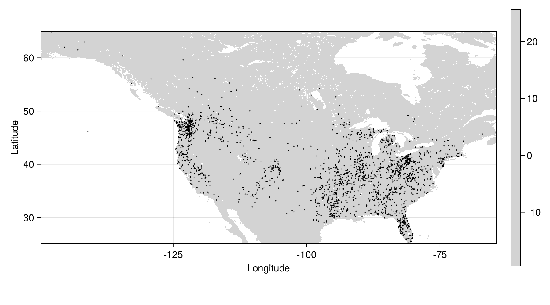
Spatial thinning
We limit the occurrences to one per grid cell, assigned to the center of the grid cell
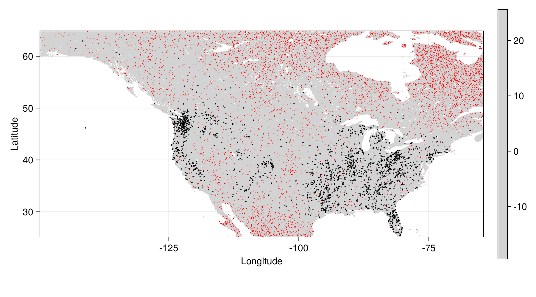
Background points generation
We generate background points proportionally to the distance away from observations, but penalize the cells that are larger due to projection
And then we sample three pseudo-absence for each occurrence:
See Barbet-Massin et al. (2012) for more on background points
Background points cleaning
We can remove all of the information that is neither a presence nor a pseudo-absence
Data overview
Preparing the responses and variables
Xpresence = hcat([bioclim_var[keys(presence_layer)] for bioclim_var in predictors]...)
ypresence = fill(true, length(presence_layer))
Xabsence = hcat([bioclim_var[keys(absence_layer)] for bioclim_var in predictors]...)
yabsence = fill(false, length(absence_layer))
X = vcat(Xpresence, Xabsence)
y = vcat(ypresence, yabsence)
The model – Naive Bayes Classifier
Prediction:
\[ P(+|x) = \frac{P(+)}{P(x)}P(x|+) \]
Decision rule:
\[ \hat y = \text{argmax}_j \, P(\mathbf{c}_j)\prod_i P(\mathbf{x}_i|\mathbf{c}_j) \]
With \(n\) instances and \(f\) features, NBC trains and predicts in \(\mathcal{O}(n\times f)\)
The model – Naive Bayes Classifier
Assumption of Gaussian distributions:
\[ P(x|+) = \text{pdf}(x, \mathcal{N}(\mu_+, \sigma_+)) \]
Cross-validation
We keep an unseen testing set – this will be used at the very end to report expected model performance
For validation, we will run k-folds
See Valavi et al. (2018) for more on cross-validation
A note on cross-validation
- All models share the same folds
-
we can compare the validation performance across experiments to select the best model
- Model performance can be compared
-
we average the relevant summary statistics over each validation set
- Testing set is only for future evaluation
-
we can only use it once and report the expected performance of the best model
Baseline performance
We need to get a sense of how difficult the classification problem is:
This uses an un-tuned model with all variables and reports the average over all validation sets. In addition, we will always use the BioClim model as a comparison.
Measures on the confusion matrix
| BioClim | NBC | |
|---|---|---|
| FPR | 0.3697 | 0.1406 |
| FNR | 0.0144 | 0.1734 |
| TPR | 0.9856 | 0.8266 |
| TNR | 0.6303 | 0.8594 |
| TSS | 0.6159 | 0.686 |
| MCC | 0.5339 | 0.6408 |
It’s a good idea to check the values for the training sets too…
Variable selection
We add variables one at a time, until the Matthew’s Correlation Coefficient stops increasing:
This method identifies 5 variables, some of which are:
Mean Temp. of Coldest Quarter
Mean Diurnal Range
Annual Precip.
Variable selection?
Constrained variable selection
VIF threshold (over the extent or over document occurrences?)
PCA for dimensionality reduction v. Whitening for colinearity removal
Potential for data leakage: data transformations don’t exist, they are just models we can train
Model with variable selection
Measures on the confusion matrix
| BioClim | NBC | BioClim (v.s.) | NBC (v.s.) | |
|---|---|---|---|---|
| FPR | 0.3697 | 0.1406 | 0.6343 | 0.0727 |
| FNR | 0.0144 | 0.1734 | 0.0056 | 0.1594 |
| TPR | 0.9856 | 0.8266 | 0.9944 | 0.8406 |
| TNR | 0.6303 | 0.8594 | 0.3657 | 0.9273 |
| TSS | 0.6159 | 0.686 | 0.3601 | 0.7679 |
| MCC | 0.5339 | 0.6408 | 0.3488 | 0.7534 |
How do we make the model better?
The NBC is a probabilistic classifier returning \(P(+|\mathbf{x})\)
The decision rule is to assign a presence when \(P(\cdot) > 0.5\)
But \(P(\cdot) > \tau\) is a far more general approach, and we can use learning curves to identify \(\tau\)
Thresholding the model
But how do we pick the threshold?

Tuned model with selected variables
Measures on the confusion matrix
| BioClim | NBC | BioClim (v.s.) | NBC (v.s.) | NBC (v.s. + tuning) | |
|---|---|---|---|---|---|
| FPR | 0.3697 | 0.1406 | 0.6343 | 0.0727 | 0.0737 |
| FNR | 0.0144 | 0.1734 | 0.0056 | 0.1594 | 0.1521 |
| TPR | 0.9856 | 0.8266 | 0.9944 | 0.8406 | 0.8479 |
| TNR | 0.6303 | 0.8594 | 0.3657 | 0.9273 | 0.9263 |
| TSS | 0.6159 | 0.686 | 0.3601 | 0.7679 | 0.7742 |
| MCC | 0.5339 | 0.6408 | 0.3488 | 0.7534 | 0.7572 |
How do we make the model better?
The NBC is a Bayesian classifier returning \(P(+|\mathbf{x})\)
The actual probability depends on \(P(+)\)
There is no reason not to also tune \(P(+)\) (jointly with other hyper-parameters)!
Joint tuning of hyper-parameters
Tuned (again) model with selected variables
Measures on the confusion matrix
| BioClim | NBC (v0) | NBC (v1) | NBC (v2) | NBC (v3) | |
|---|---|---|---|---|---|
| FPR | 0.3697 | 0.1406 | 0.0727 | 0.0737 | 0.0735 |
| FNR | 0.0144 | 0.1734 | 0.1594 | 0.1521 | 0.1521 |
| TPR | 0.9856 | 0.8266 | 0.8406 | 0.8479 | 0.8479 |
| TNR | 0.6303 | 0.8594 | 0.9273 | 0.9263 | 0.9265 |
| TSS | 0.6159 | 0.686 | 0.7679 | 0.7742 | 0.7744 |
| MCC | 0.5339 | 0.6408 | 0.7534 | 0.7572 | 0.7575 |
Tuned model performance
We can retrain over all the training data
Estimated performance
| Final model | |
|---|---|
| FPR | 0.0769 |
| FNR | 0.1432 |
| TPR | 0.8568 |
| TNR | 0.9231 |
| TSS | 0.7799 |
| MCC | 0.7593 |
Acceptable bias
false positives: we expect that our knowledge of the distribution is incomplete, and this is why we train a model
false negatives: wrong observations (positive in the data) may be identified by the model (negative prediction)
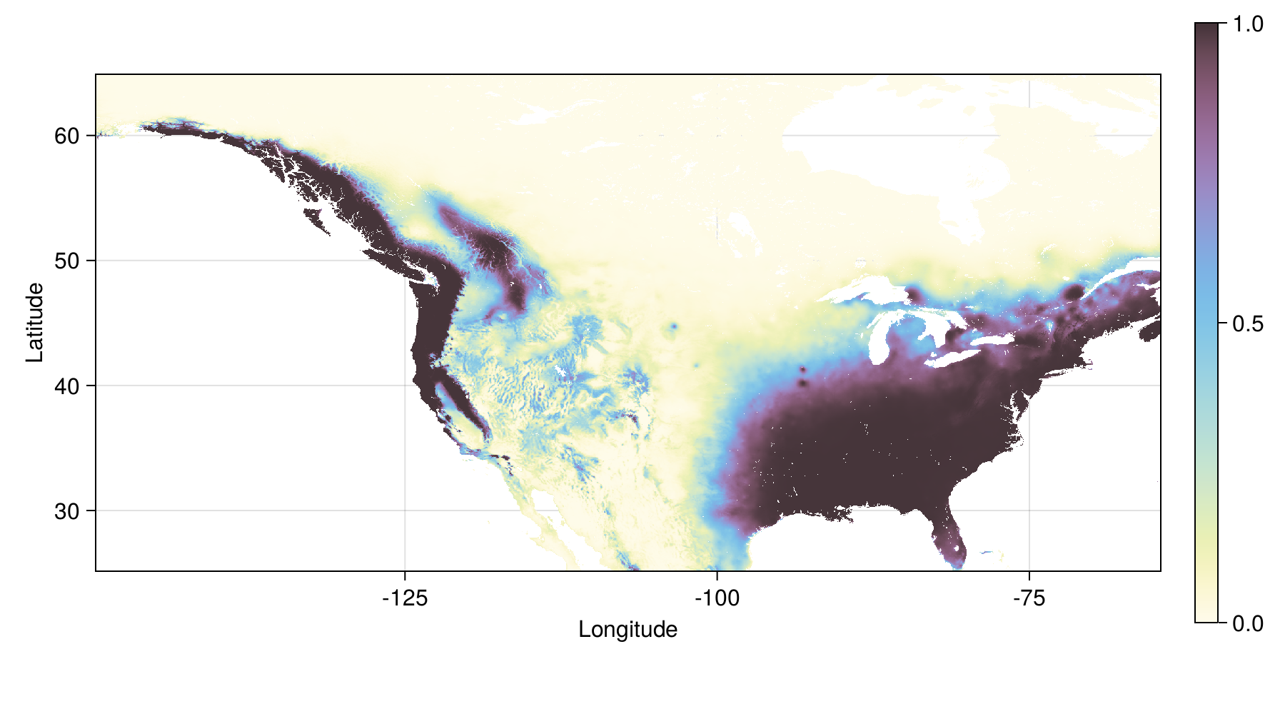
Prediction for each pixel
prediction = similar(temperature, Float64)
variability = similar(temperature, Float64)
uncertainty = similar(temperature, Float64)
Threads.@threads for k in keys(prediction)
pred_k = [p[k] for p in predictors[available_variables]]
bootstraps = [
samplemodel(pred_k)
for samplemodel in samplemodels
]
prediction[k] = finalmodel(pred_k)
variability[k] = iqr(bootstraps)
uncertainty[k] = entropy(prediction[k])
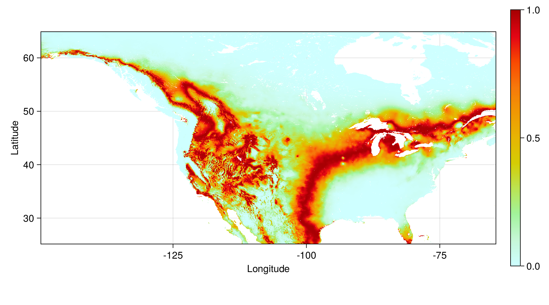
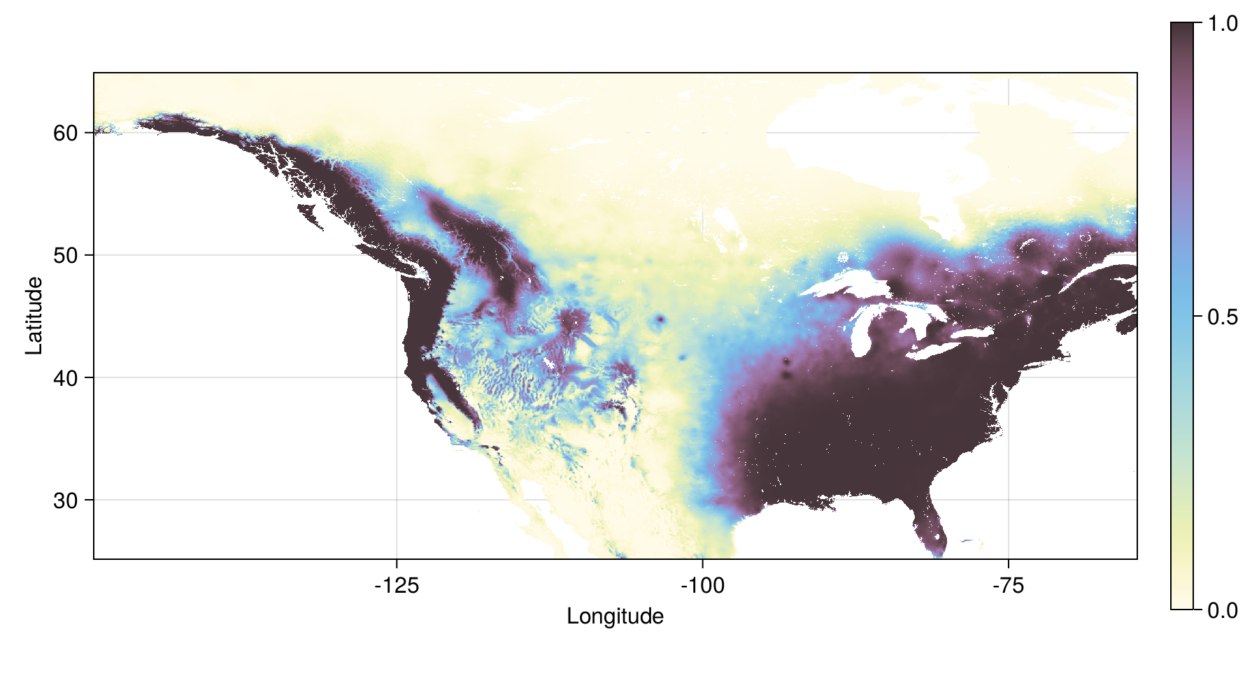
endTuned model - prediction
Tuned model - variability in output
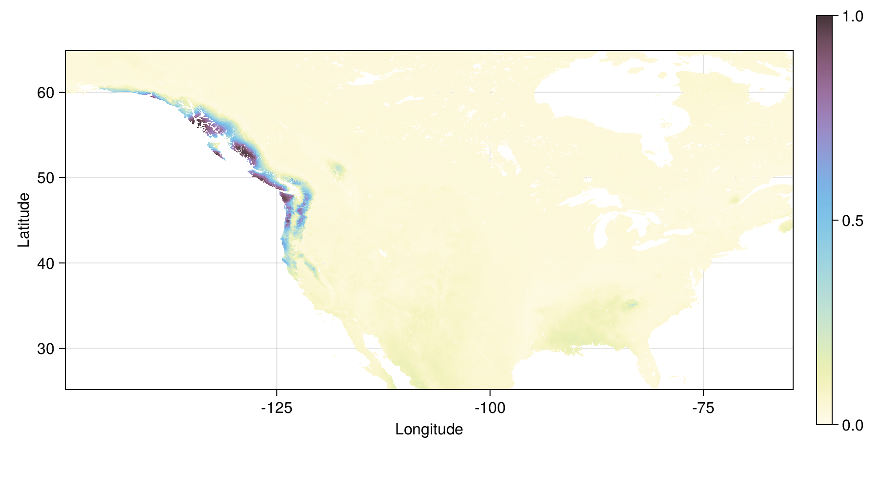
IQR for 50 bootstrap replicates
Tuned model - entropy in probability
Entropy (in bits) of the NBC probability
Tuned model - range
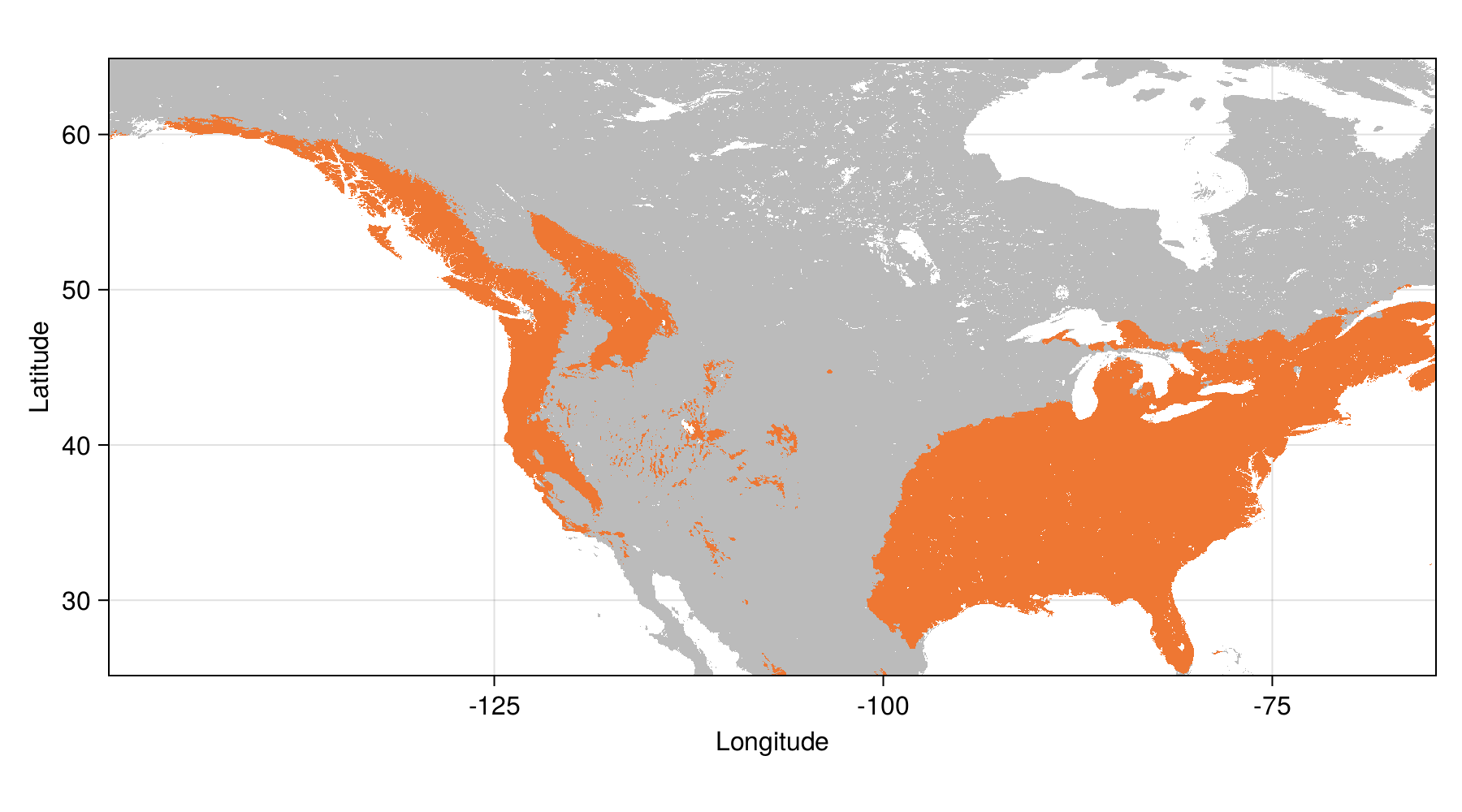
Probability > 0.5
Predicting the predictions?
Shapley values (Monte-Carlo approximation): if we mix the variables across two observations, how important is the \(i\)-th variable?
Expresses “importance” as an additive factor on top of the average prediction (here: average prob. of occurrence)
Calculation of the Shapley values
shapval = [similar(first(predictors), Float64) for i in eachindex(available_variables)]
Threads.@threads for k in keys(shapval[1])
x = [p[k] for p in predictors[available_variables]]
for i in axes(shapval, 1)
shapval[i][k] = shapleyvalues(finalmodel, tX[:,available_variables], x, i; M=50)
if isnan(shapval[i][k])
shapval[i][k] = 0.0
end
end
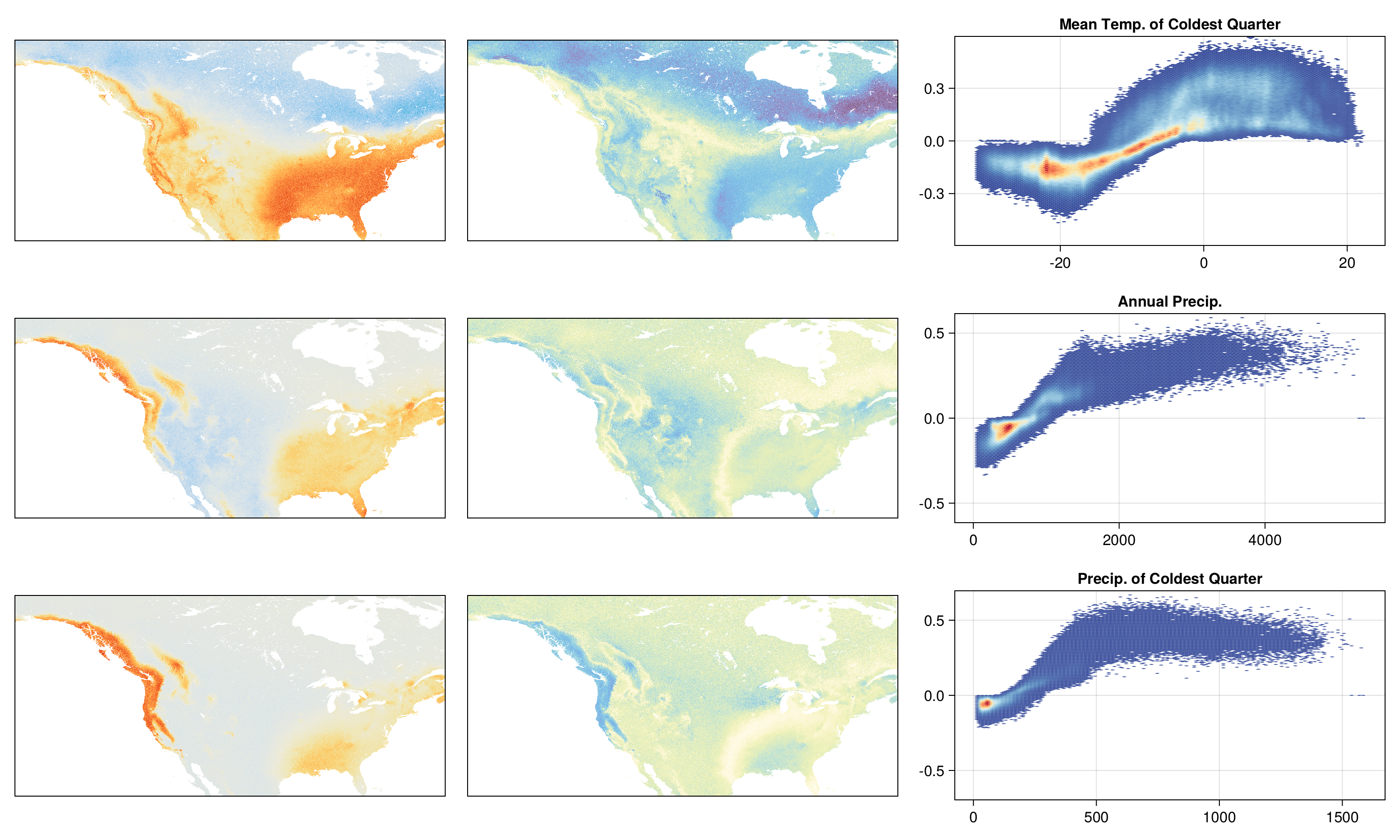
endImportance of variables
varimp = sum.(map(abs, shapval))
varimp ./= sum(varimp)
shapmax = mosaic(argmax, map(abs, shapval[sortperm(varimp; rev=true)]))
for v in sortperm(varimp, rev=true)
    vname = variables[available_variables[v]][2]
    vctr = round(Int, varimp[v]*100)
    println("$(vname) - $(vctr)%")
end
Mean Temp. of Coldest Quarter - 38%
Annual Precip. - 20%
Precip. of Coldest Quarter - 18%
Mean Diurnal Range - 12%
Precip. Seasonality - 11%There is a difference between contributing to model performance and contributing to model explainability
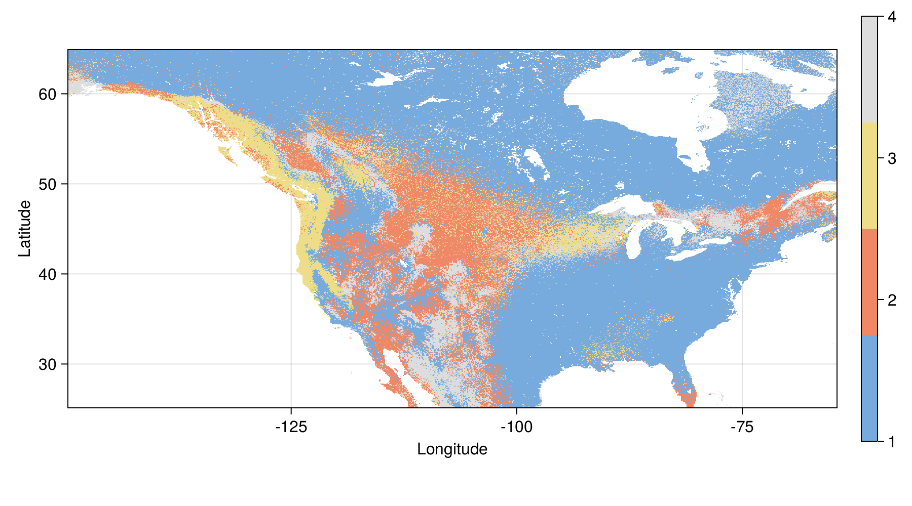
Top three variables
Most determinant predictor
Future predictions
relevant variables will remain the same
relevant \(P(+)\) will remain the same
relevant threshold for presences will remain the same
Future climate data (ca. 2070)
Future climate prediction
Tuned model - future prediction
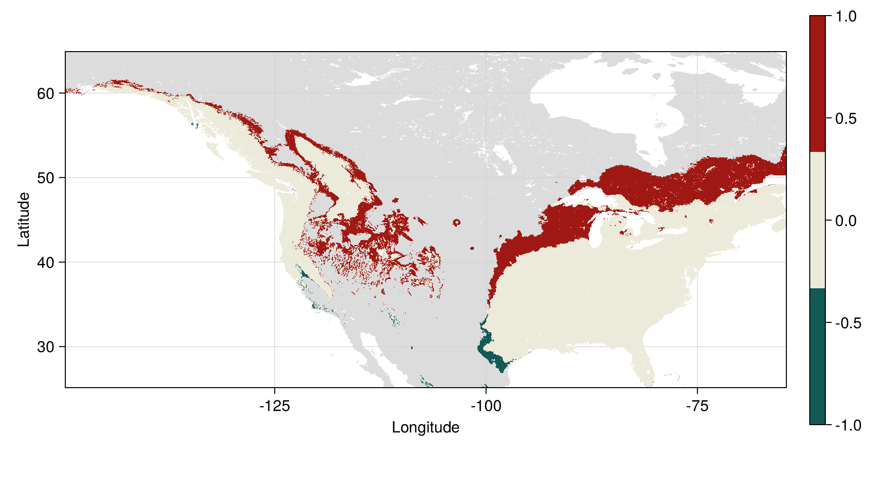
Loss and gain in distribution
| Change | Area (10⁶ km²) |
|---|---|
| Expansion | 1.732 |
| No change | 4.659 |
| Loss | 0.093 |
Tuned model - future range change
But wait…
What do you think the species was?
Human in the loop v. Algorithm in the loop
Take-home
building a model is incremental
each step adds arbitrary decisions we can control for, justify, or live with
we can provide explanations for every single prediction
free online textbook (in development) at
https://tpoisot.github.io/DataSciForBiodivSci/
References

Barbet-Massin, M., Jiguet, F., Albert, C.H. & Thuiller, W. (2012). Selecting pseudo-absences for species distribution models: how, where and how many? Methods in Ecology and Evolution, 3, 327–338.
Beery, S., Cole, E., Parker, J., Perona, P. & Winner, K. (2021). Species distribution modeling for machine learning practitioners: A review. ACM SIGCAS Conference on Computing and Sustainable Societies (COMPASS).
Dansereau, G. & Poisot, T. (2021). SimpleSDMLayers.jl and GBIF.jl: A framework for species distribution modeling in julia. Journal of Open Source Software, 6, 2872.
Karger, D.N., Schmatz, D.R., Dettling, G. & Zimmermann, N.E. (2020). High-resolution monthly precipitation and temperature time series from 2006 to 2100. Scientific Data, 7.
Tuanmu, M.-N. & Jetz, W. (2014). A global 1-km consensus land-cover product for biodiversity and ecosystem modelling. Global Ecology and Biogeography, 23, 1031–1045.
Valavi, R., Elith, J., Lahoz-Monfort, J.J. & Guillera-Arroita, G. (2018). blockCV: An r package for generating spatially or environmentally separated folds for k-fold cross-validation of species distribution models. Methods in Ecology and Evolution, 10, 225–232.