5 Supervised classification
In the previous chapters, we have focused on efforts on regression models, which is to say models that predict a continuous response. In this chapter, we will introduce the notion of classification, which is the prediction of a discrete variable representing a category. There are a lot of topics we need to cover before we can confidently come up with a model for classification, and so this chapter is part of a series. We will first introduce the idea of classification; in ?sec-variable-selection, we will explore techniques to fine-tune the set of variables we use for prediction; in Chapter 7, we will think about predictions of classes as probabilities, and generalize these ideas and think about learning curves; finally, in Chapter 8, we will think about variables a lot more, and introduce elements of model interpretability.
5.1 The problem: distribution of an endemic species
Throughout these chapters, we will be working on a single problem, which is to predict the distribution of the Corsican nuthatch, Sitta whiteheadi. The Corsican nuthatch is endemic to Corsica, and its range has been steadily shrinking over time due to loss of habitat through human activity, including fire, leading to it being classified as “vulnerable to extinction” by the International Union for the Conservation of Nature. Barbet-Massin and Jiguet (2011) nevertheless show that the future of this species is not necessarily all gloom and doom, as climate change is not expected to massively affect its distribution.
Species Distribution Modeling (SDM; Elith and Leathwick (2009)), also known as Ecological Niche Modeling (ENM), is an excellent instance of ecologists doing applied machine learning already, as Beery et al. (2021) rightfully pointed out. In fact, the question of fitness-for-purpose, which we discussed in previous chapters (for example in Section 4.4.3), has been covered in the SDM literature (Guillera-Arroita et al. 2015). In these chapters, we will fully embrace this idea, and look at the problem of predicting where species can be as a data science problem. In the next chapters, we will converge again on this problem as an ecological one. Being serious our data science practices when fitting a species distribution model is important: Chollet Ramampiandra et al. (2023) make the important point that it is easy to overfit more complex models, at which point they cease outperforming simple statistical models.
Because this chapter is the first of a series, we will start by building a bare-bones model on ecological first principles. This is an important step. The rough outline of a model is often indicative of how difficult the process of training a really good model will be. But building a good model is an iterative process, and so we will start with a very simple model and training strategy, and refine it over time. In this chapter, the purpose is less to have a very good training process; it is to familiarize ourselves with the task of classification.
We will therefore start with a blanket assumption: the distribution of species is something we can predict based on temperature and precipitation. We know this to be important for plants (Clapham et al. 1935) and animals (Whittaker 1962), to the point where the relationship between mean temperature and annual precipitation is how we find delimitations between biomes. If you need to train a lot of models on a lot of species, temperature and precipitation are not the worst place to start (Berteaux 2014).
Consider our dataset for a minute. In order to predict the presence of a species, we need information about where the species has been observed; this we can get from the Global Biodiversity Information Facility. We need information about where the species has not been observed; this is usually not directly available, but there are ways to generate background points that are a good approximation of this (Hanberry, He, and Palik 2012; Barbet-Massin et al. 2012). All of these data points come in the form \((\text{lat.}, \text{lon.}, y)\), which give a position in space, as well as \(y = \{+,-\}\) (the species is present or absent!) at this position.
To build a model with temperature and precipitation as inputs, we need to extract the temperature and precipitation at all of these coordinates. We will use the CHELSA2 dataset (Karger et al. 2017), at a resolution of 30 seconds of arc. WorldClim2 (Fick and Hijmans 2017) is also appropriate, but is known to have some artifacts.
The predictive task we want to complete is to get a predicted presence or absence \(\hat y = \{+,-\}\), from a vector \(\mathbf{x}^\top = [\text{temp.} \quad \text{precip.}]\). This specific task is called classification, and we will now introduce some elements of theory.
5.2 What is classification?
Classification is the prediction of a qualitative response. In Chapter 2, for example, we predicted the class of a pixel, which is a qualitative variable with levels \(\{1, 2, \dots, k\}\). This represented an instance of unsupervised learning, as we had no a priori notion of the correct class of the pixel. When building SDMs, by contrast, we often know where species are, and we can simulate “background points”, that represent assumptions about where the species are not. For this series of chapters, the background points have been generated by sampling preferentially the pixels that are farther away from known presences of the species.
When working on \(\{+,-\}\) outcomes, we are specifically performing binary classification. Classification can be applied to more than two levels.
In short, our response variable has levels \(\{+, -\}\): the species is there, or it is not – we will challenge this assumption later in the series of chapters, but for now, this will do. The case where the species is present is called the positive class, and the case where it is absent is the negative class. We tend to have really strong assumptions about classification already. For example, monitoring techniques using environmental DNA (e.g. Perl et al. 2022) are a classification problem: the species can be present or not, \(y = \{+,-\}\), and the test can be positive of negative \(\hat y = \{+,-\}\). We would be happy in this situation whenever \(\hat y = y\), as it means that the test we use has diagnostic value. This is the essence of classification, and everything that follows is more precise ways to capture how close a test comes from this ideal scenario.
5.2.1 Separability
A very important feature of the relationship between the features and the classes is that, broadly speaking, classification is much easier when the classes are separable. Separability (often linear separability) is achieved when, if looking at some projection of the data on two dimensions, you can draw a line that separates the classes (a point in a single dimension, a plane in three dimension, and so on and so forth). For reasons that will become clear in ?sec-variableselection-curse, simply adding more predictors is not necessarily the right thing to do.
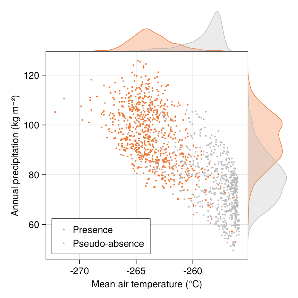
In Figure 5.1, we can see the temperature (in degrees) for locations with recorded presences of Corsican nuthatches, and for locations with assumed absences. These two classes are not quite linearly separable alongside this single dimension (maybe there is a different projection of the data that would change this; we will explore one in ?sec-variable-selection), but there are still some values at which our guess for a class changes. For example, at a location with a temperature colder than 1°C, presences are far more likely. For a location with a temperature warmer than 5°C, absences become overwhelmingly more likely. The locations with a temperature between 0°C and 5°C can go either way.
5.2.2 The confusion table
Evaluating the performance of a classifier (a classifier is a model that performs classification) is usually done by looking at its confusion table, which is a contingency table of the form
\[ \begin{pmatrix} \text{TP} & \text{FP}\\ \text{FN} & \text{TN} \end{pmatrix} \,. \tag{5.1}\]
This can be stated as “counting the number of times each pair of (prediction, observation occurs)”, like so:
\[ \begin{pmatrix} |\hat +, +| & |\hat +, -|\\ |\hat -, +| & |\hat -, -| \end{pmatrix} \,. \tag{5.2}\]
The four components of the confusion table are the true positives (TP; correct prediction of \(+\)), the true negatives (TN; correct prediction of \(-\)), the false positives (FP; incorrect prediction of \(+\)), and the false negatives (FN; incorrect prediction of \(-\)). Quite intuitively, we would like our classifier to return mostly elements in TP and TN: a good classifier has most elements on the diagonal, and off-diagonal elements as close to zero as possible (the proportion of predictions on the diagonal is called the accuracy, and we will spend Section 5.2.4 discussing why it is not such a great measure).
As there are many different possible measures on this matrix, we will introduce them as we go. In this section, it it more important to understand how the matrix responds to two important features of the data and the model: balance and bias.
Balance refers to the proportion of the positive class. Whenever this balance is not equal to 1/2 (there are as many positives as negative cases), we are performing imbalanced classification, which comes with additional challenges; few ecological problems are balanced.
5.2.3 The no-skill classifier
There is a specific hypothetical classifier, called the no-skill classifier, which guesses classes at random as a function of their proportion. It turns out to have an interesting confusion matrix! If we note \(b\) the proportion of positive classes, the no-skill classifier will guess \(+\) with probability \(b\), and \(-\) with probability \(1-b\). Because these are also the proportion in the data, we can write the adjacency matrix as
\[ \begin{pmatrix} b^2 & b(1-b)\\ (1-b)b & (1-b)^2 \end{pmatrix} \,. \tag{5.3}\]
The proportion of elements that are on the diagonal of this matrix is \(b^2 + (1-b)^2\). When \(b\) gets lower, this value actually increases: the more difficult a classification problem is, the more accurate random guesses look like. This has a simple explanation, which we expand Section 5.2.4 : when most of the cases are negative, if you predict a negative case often, you will by chance get a very high true negative score. For this reason, measures of model performance will combine the positions of the confusion table to avoid some of these artifacts.
An alternative to the no-skill classifier is the coin-flip classifier, in which classes have their correct prevalence \(b\), but the model picks at random (i.e. with probability \(1/2\)) within these classes.
Bias refers to the fact that a model can recommend more (or fewer) positive or negative classes than it should. An extreme example is the zero-rate classifier, which will always guess the most common class, and which is commonly used as a baseline for imbalanced classification. A good classifier has high skill (which we can measure by whether it beats the no-skill classifier for our specific problem) and low bias. In this chapter, we will explore different measures on the confusion table the inform us about these aspects of model performance, using the Naive Bayes Classifier.
5.2.4 A note on accuracy
It is tempting to use accuracy to measure how good a classifier is, because it makes sense: it quantifies how many predictions are correct. But a good accuracy can hide a very poor performance. Let’s think about an extreme case, in which we want to detect an event that happens with prevalence \(0.05\). Out of 100 predictions, the confusion matrix of this model would be
\[ \begin{pmatrix} 0 & 0 \\ 5 & 95 \end{pmatrix} \,. \]
The accuracy of this classifier would be \(0.95\), which seems extremely high! This is because prevalence is extremely low, and so most of the predictions are about the negative class: the model is on average really good, but is completely missing the point when it comes to making interesting predictions.
In fact, even a classifier that would not be that extreme would be mis-represented if all we cared about was the accuracy. If we take the case of the no-skill classifier, the accuracy is given by \(b^2 + (1-b)^2\), which is an inverted parabola that is maximized for \(b \approx 0\) – a model guessing at random will appear better when the problem we want to solve gets more difficult.
This is an issue inherent to accuracy: it can tell you that a classifier is bad (when it is low), but it cannot really tell you when a classifier is good, as no-skill (or worse-than-no-skill) classifiers can have very high values. It remains informative as an a posteriori measure of performance, but only after using reliable measures to ensure that the model means something.
5.3 The Naive Bayes Classifier
The Naive Bayes Classifier (NBC) is my all-time favorite classifier. It is built on a very simple intuition, works with almost no data, and more importantly, often provides an annoyingly good baseline for other, more complex classifiers to meet. That NBC works at all is counter-intuitive (Hand and Yu 2001). It assumes that all variables are independent, it works when reducing the data to a simpler distribution, and although the numerical estimate of the class probability can be somewhat unstable, it generally gives good predictions. NBC is the data science equivalent of saying “eh, I reckon it’s probably this class” and somehow getting it right 95% of the case [there are, in fact, several papers questioning why NBC works so well; see e.g. Kupervasser (2014)].
5.3.1 How the NBC works
In Figure 5.1, what is the most likely class if the temperature is 12°C? We can look at the density traces on top, and say that because the one for presences is higher, we would be justified in guessing that the species is present. Of course, this is equivalent to saying that \(P(12^\circ C | +) > P(12^\circ C | -)\). It would appear that we are looking at the problem in the wrong way, because we are really interested in \(P(+ | 12^\circ C)\), the probability that the species is present knowing that the temperature is 12°C.
Using Baye’s theorem, we can re-write our goal as
\[ P(+|x) = \frac{P(+)}{P(x)}P(x|+) \,, \tag{5.4}\]
where \(x\) is one value of one feature, \(P(x)\) is the probability of this observation (the evidence, in Bayesian parlance), and \(P(+)\) is the probability of the positive class (in other words, the prior). So, this is where the “Bayes” part comes from.
But why is NBC naïve?
In Equation 5.4, we have used a single feature \(x\), but the problem we want to solve uses a vector of features, \(\mathbf{x}\). These features, statisticians will say, will have covariance, and a joint distribution, and many things that will challenge the simplicity of what we have written so far. These details, NBC says, are meaningless.
NBC is naïve because it makes the assumptions that the features are all independent. This is very important, as it means that \(P(+|\mathbf{x}) \propto P(+)\prod_i P(\mathbf{x}_i|+)\) (by the chain rule). Note that this is not a strict equality, as we need to divide by the evidence. But the evidence is constant across all classes, and so we do not need to measure it to get an estimate of the score for a class.
To generalize our notation, the score for a class \(\mathbf{c}_j\) is \(P(\mathbf{c}_j)\prod_i P(\mathbf{x}_i|\mathbf{c}_j)\). In order to decide on a class, we apply the following rule:
\[ \hat y = \text{argmax}_j \, P(\mathbf{c}_j)\prod_i P(\mathbf{x}_i|\mathbf{c}_j) \,. \tag{5.5}\]
In other words, whichever class gives the higher score, is what the NBC will recommend for this instance \(\mathbf{x}\). In Chapter 7, we will improve upon this model by thinking about the evidence \(P(\mathbf{x})\), but as you will see, this simple formulation will already prove frightfully effective.
5.3.2 How the NBC learns
There are two unknown quantities at this point. The first is the value of \(P(+)\) and \(P(-)\). These are priors, and are presumably important to pick correctly. In the spirit of iterating rapidly on a model, we can use two starting points: either we assume that the classes have the same probability, or we assume that the representation of the classes (the balance of the problem) is their prior. More broadly, we do not need to think about \(P(-)\) too much, as it is simply \(1-P(+)\), since the “state” of every single observation of environmental variables is either \(+\) or \(-\).
The most delicate problem is to figure out \(P(x|c)\), the probability of the observation of the variable when the class is known. There are variants here that will depend on the type of data that is in \(x\); as we work with continuous variables, we will rely on Gaussain NBC. In Gaussian NBC, we will consider that \(x\) comes from a normal distribution \(\mathcal{N}(\mu_{x,c},\sigma_{x,c})\), and therefore we simply need to evaluate the probability density function of this distribution at the point \(x\). Other types of data are handled in the same way, with the difference that they use a different set of distributions.
Therefore, the learning stage of NBC is extremely quick: we take the mean and standard deviation of the values, split by predictor and by class, and these are the parameters of our classifier. By contrast to the linear regression approach we worked with in Chapter 3, the learning phase only involves a single epoch: measuring the mean and standard deviation.
5.4 Application: a baseline model of the Corsican nuthatch
In this section, we will have a look at the temperature and precipitation data from Figure 5.1, and come up with a first version of our classifier.
5.4.1 Training and validation strategy
To evaluate our model, as we discussed in Chapter 4, we will keep a holdout testing set, that will be composed of 20% of the observations. In this chapter, we will not be using these data, because in order to use them as a stand-in for future predictions, it is important that the model only sees them once (this will happen at the end of Chapter 7). Therefore, for the next chapters, we will limit ourselves to an evaluation of the model performance based on the average values of the performance measure we picked as the most informative, calculated on the validation datasets. In this chapter, we will rely on Monte-Carlo cross validation (MCCV; see Section 4.3.5), using 50 replicates. In the following chapters, we will revert to using k-folds cross-validation, but using MCCV here is a good enough starting point.
In order to see how good our model really is, we will also compare its performances to the no-skill classifier. This is almost never a difficult classifier to outperform, but this nevertheless provides a good indication of whether our model works at all. In subsequent chapters, we will introduce a slightly more domain-specific model to provide a baseline that would look like an actual model we would like to out-perform.
5.4.2 Performance evaluation of the model
In order to get a sense of the performance of our model, we will need to decide on a performance measure. This is an important step, as we will use the average value of this measure on the validation data to decide on the best model before reporting the expected performance. If we pick a measure that is biased, we will therefore use a model that is biased. Following Chicco and Jurman (2020) and Jurman, Riccadonna, and Furlanello (2012), we will use the Matthew’s Correlation Coefficient (MCC) as the “main” measure to evaluate the performance of a model (we will return to other alternative measures in Chapter 7).
The MCC is defined as
\[ \frac{\text{TP}\times \text{TN} - \text{FP}\times \text{FN}}{\sqrt{(\text{TP}+\text{FP})\times (\text{TP}+\text{FN})\times (\text{TN}+\text{FP})\times (\text{TN}+\text{FN})}} \,. \]
The MCC is a correlation coefficient (specifically, the Pearson product-moment correlation on a contingency table; Powers (2020)), meaning that it returns values in \([-1, 1]\). A negative value indicates perfectly wrong predictions, a value of 0 indicates no-skill, and a value of 1 indicates perfect predictions. Therefore, if we pick the model with the highest MCC, we are likely to pick the best possible model.
In addition to reporting the MCC, we will also look at values that inform us on the type of biases in the model, namely the positive and negative predictive values. These values, respectively \(\text{TP}/(\text{TP}+\text{FP})\) and \(\text{TN}/(\text{TN}+\text{FN})\), measure how likely a prediction of, respectively, presence and absence, are. These range in \([0,1]\), and values of one indicate a better performance of the model.
Why not pick one of these instead of the MCC? Well, all modeling is compromise; we don’t want a model to become too good at predicting absences, to the point where prediction about presences would become meaningless. Selecting models on the basis of a measure that only emphasizes one outcome is a risk that we shouldn’t be willing to take. For this reason, measures that are good at optimizing the value of a negative and a positive predictions are far better representations of the performance of a model. The MCC does just this.
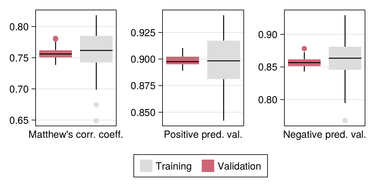
The output of cross-validation is given in Figure 5.2 (and compared to the no-skill classifier in Table 5.1). As we are satisfied with the model performance, we can re-train it using all the data (but not the part used for testing) in order to make our first series of predictions.
| Measure | Training | Validation | No-skill |
|---|---|---|---|
| Accuracy | 0.879 | 0.882 | 0.505 |
| NPV | 0.857 | 0.861 | 0.449 |
| PPV | 0.899 | 0.9 | 0.551 |
| MCC | 0.757 | 0.762 | 0.0 |
5.4.3 The decision boundary
Now that the model is trained, we can take a break in our discussion of its performance, and think about why it makes a specific classification in the first place. Because we are using a model with only two input features, we can generate a grid of variables, and the ask, for every point on this grid, the classification made by our trained model. This will reveal the regions in the space of parameters where the model will conclude that the species is present.
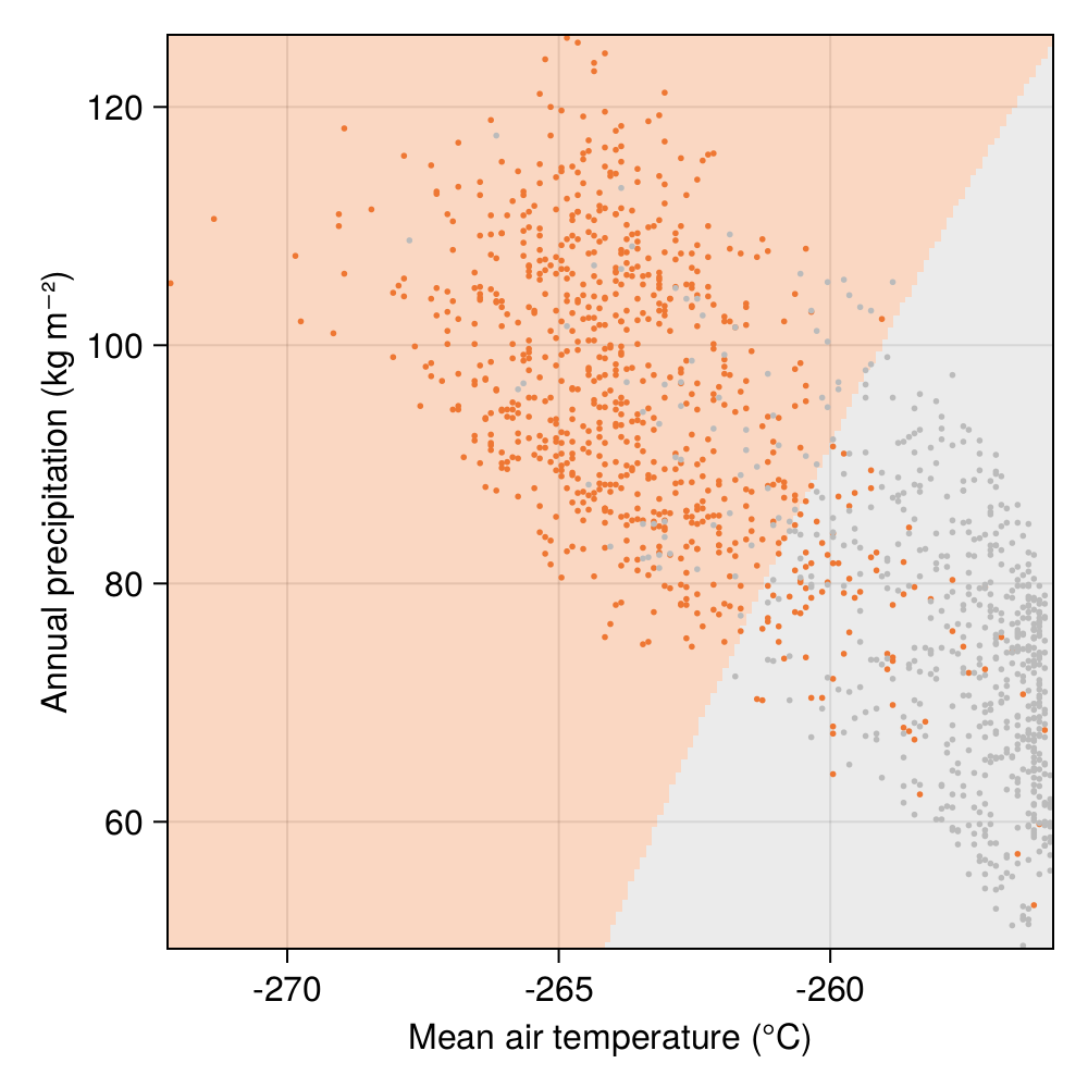
The output of this simulation is given in Figure 5.3. Of course, in a model with more features, we would need to adapt our visualisations, but because we only use two features here, this image actually gives us a complete understanding of the model decision process. Think of it this way: even if we lose the code of the model, we could use this figure to classify any input made of a temperature and a precipitation, and read what the model decision would have been.
The line that separates the two classes is usually refered to as the “decision boundary” of the classifier: crossing this line by moving in the space of features will lead the model to predict another class at the output. In this instance, as a consequence of the choice of models and of the distribution of presence and absences in the environmental space, the decision boundary is not linear.
Take a minute to think about which places are more likely to have lower temperatures on an island. Is there an additional layer of geospatial information we could add that would be informative?
It is interesting to compare Figure 5.3 with, for example, the distribution of the raw data presented in Figure 5.1. Although we initially observed that temperature was giving us the best chance to separate the two classes, the shape of the decision boundary suggests that our classifier is considering that Corsican nuthatches enjoy colder climates with more rainfall.
5.4.4 Visualizing the trained model
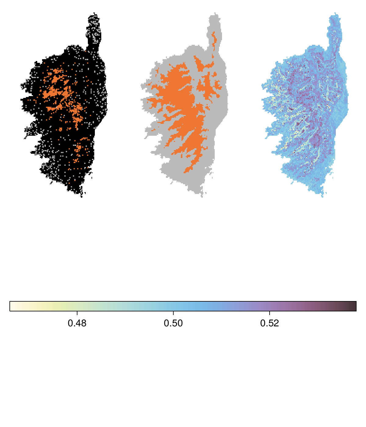
We can now go through all of the pixels in the island of Corsica, and apply the model to predict the presence of Sitta whiteheadi. This result is reported in Figure 5.4. In order to have a little more information about where the predictions can be trusted, we also perform a little bit of bootstrapping: in this approach, we re-train the model using samples with replacement of the training data (500 times), and apply this batch of models, and measure the proportion of times they give the same prediction as the model trained on all the data. When this is higher, this indicates that the prediction is robust with regard to the training dataset.
5.4.5 What is an acceptable model?
When comparing the prediction to the spatial distribution of occurrences (Figure 5.4), it appears that the model identifies an area in the northwest where the species is likely to be present, despite limited observations. This might result in more false positives, but this is the purpose of running this model – if the point data were to provide us with a full knowledge of the range, there would be no point in running the model. For this reason, it is very important to nuance our interpretation of what a false-positive prediction really is. We will get back to this discussion in the next chapters, when adding more complexity to the model.
5.5 Conclusion
In this chapter, we introduced the Naive Bayes Classifier as a model for classification, and applied it to a data of species occurrence, in which we predicted the potential presence of the species using temperature and classification. Through cross-validation, we confirmed that this model gave a good enough performance (Figure 5.2), looked at the decisions that were being made by the trained model (Figure 5.3), and finally mapped the prediction and their uncertainty in space (Figure 5.4). In the next chapter, we will improve upon this model by looking at techniques to select and transform variables.