| Step | Loss (training) | Loss (testing) | β₀ | β₁ |
|---|---|---|---|---|
| 1 | 3.92114 | 3.18785 | 0.4 | 0.2 |
| 10 | 2.99934 | 2.3914 | 0.487395 | 0.226696 |
| 30 | 1.72775 | 1.31211 | 0.640263 | 0.271814 |
| 100 | 0.536207 | 0.373075 | 0.907004 | 0.337644 |
| 300 | 0.392477 | 0.308264 | 1.03855 | 0.311011 |
| 1000 | 0.326848 | 0.253939 | 1.11195 | 0.110083 |
| 3000 | 0.225623 | 0.167897 | 1.25704 | -0.311373 |
| 10000 | 0.164974 | 0.119597 | 1.4487 | -0.868105 |
| 20000 | 0.162808 | 0.118899 | 1.48864 | -0.984121 |
3 Gradient descent
As we progress into this book, the process of delivering a trained model is going to become more and more complex. In Chapter 2, we worked with a model that did not really require training (but did require to pick the best hyper-parameter). In this chapter, we will only increase complexity very slightly, by considering how we can train a model when we have a reference dataset to compare to.
Doing do will require to introduce several new concepts, and so the “correct” way to read this chapter is to focus on the high-level process. The problem we will try to solve (which is introduced in Section 3.2) is very simple; in fact, the empirical data looks more fake than many simulated datasets!
3.1 A digression: what is a trained model?
Models are data. When a model is trained, it represents a series of measurements (its parameters), taken on a representation of the natural world (the training data), through a specific instrument (the model itself, see e.g. Morrison and Morgan 1999). A trained model is, therefore, capturing our understanding of a specific situation we encountered. We need to be very precise when defining what, exactly, a model describes. In fact, we need to take a step back and try to figure out where the model stops.
As we will see in this chapter, then in Chapter 4, and finally in Chapter 7, the fact of training a model means that there is a back and forth between the algorithm we train, the data we use for training, and the criteria we set to define the performance of the trained model. The algorithm bound to its dataset is the machine we train in machine learning.
Therefore, a trained model is never independent from its training data: they describe the scope of the problem we want to address with this model. In Chapter 2, we ended up with a machine (the trained k-means algorithm) whose parameters (the centroids of the classes) made sense in the specific context of the training data we used; applied to a different dataset, there are no guarantees that our model would deliver useful information.
For the purpose of this book, we will consider that a model is trained when we have defined the algorithm, the data, the measure through which we will evaluate the model performance, and then measured the performance on a dataset built specifically for this task. All of these elements are important, as they give us the possibility to explain how we came up with the model, and therefore, how we made the predictions. This is different from reasoning about why the model is making a specific prediction (we will discuss this in Chapter 8), and is more related to explaining the process, the “outer core” of the model. As you read this chapter, pay attention to these elements: what algorithm are we using, on what data, how do we measure its performance, and how well does it perform?
3.2 The problem: how many interactions in a food web?
One of the earliest observation that ecologists made about food webs is that when there are more species, there are more interactions. A remarkably insightful crowd, food web ecologists. Nevertheless, it turns out that this apparently simple question had received a few different answers over the years.
The initial model was proposed by Cohen and Briand (1984): the number of interactions \(L\) scales linearly with the number of species \(S\). After all, we can assume that when averaging over many consumers, there will be an average diversity of resources they consume, and so the number of interactions could be expressed as \(L \approx b\times S\).
Not so fast, said Martinez (1992). When we start looking a food webs with more species, the increase of \(L\) with regards to \(S\) is superlinear. Thinking in ecological terms, maybe we can argue that consumers are flexible, and that instead of sampling a set number of resources, they will sample a set proportion of the number of consumer-resource combinations (of which there are \(S^2\)). In this interpretation, \(L \approx b\times S^2\).
But the square term can be relaxed; and there is no reason not to assume a power law, with \(L\approx b\times S^a\). This last formulation has long been accepted as the most workable one, because it is possible to approximate values of its parameters using other ecological processes (Brose et al. 2004).
The “reality” (i.e. the relationship between \(S\) and \(L\) that correctly accounts for ecological constraints, and fit the data as closely as possible) is a little bit different than this formula (MacDonald, Banville, and Poisot 2020). But for the purpose of this chapter, figuring out the values of \(a\) and \(b\) from empirical data is a very instructive exercise.
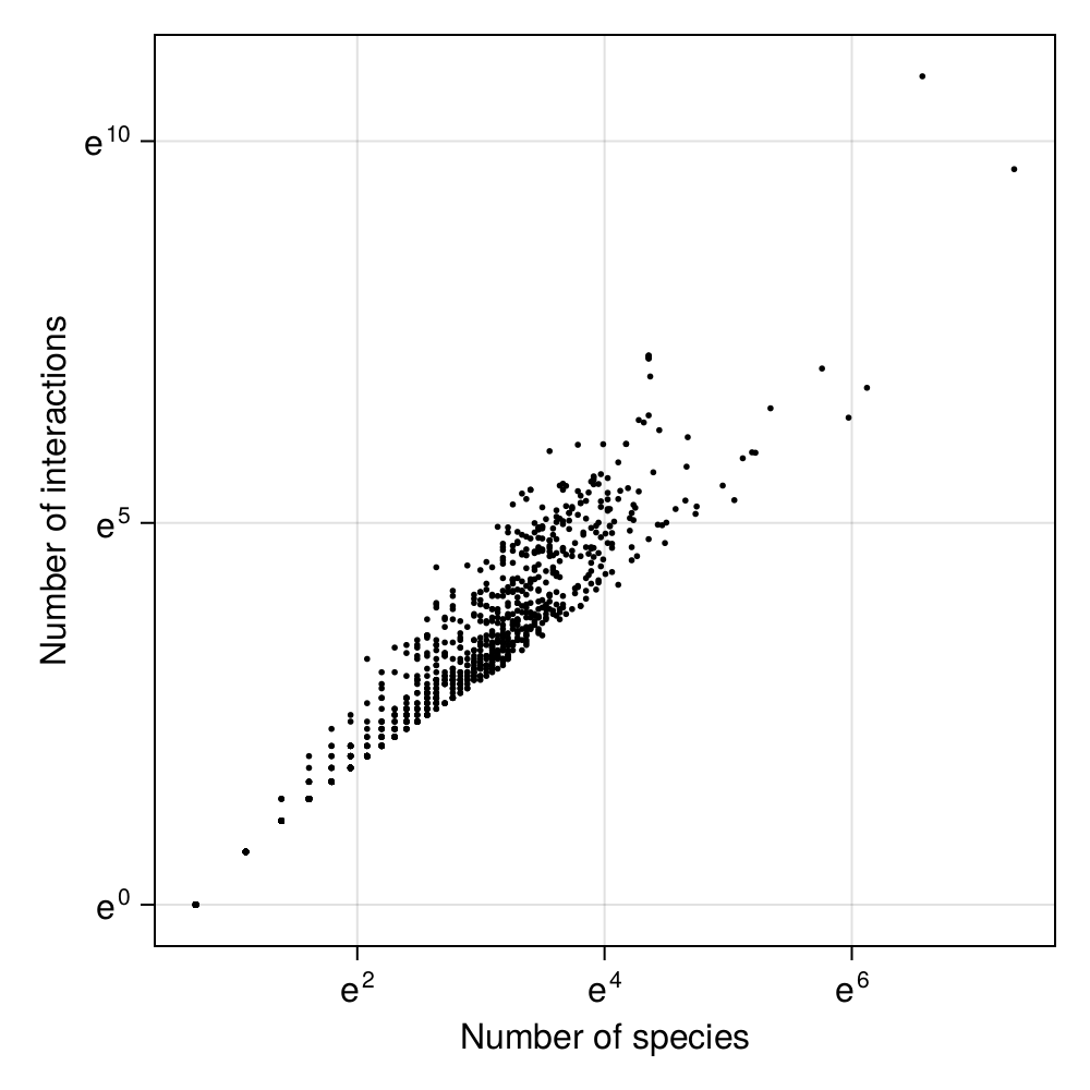
In Figure 3.1, we can check that there is a linear relationship between the natural log of the number of species and the natural log of the number of links. This is not surprising! If we assume that \(L \approx b\times S^a\), then we can take the log of both sides, and we get \(\text{log}\, L \approx a \times \text{log}\, S + \text{log}\,b\). This is linear model, and so we can estimate its parameters using linear regression!
3.3 Gradient descent
Gradient descent is built around a remarkably simple intuition: knowing the formula that gives rise to our prediction, and the value of the error we made for each point, we can take the derivative of the error with regards to each parameter, and this tells us how much this parameter contributed to the error. Because we are taking the derivative, we can futher know whether to increase, or decrease, the value of the parameter in order to make a smaller error next time.
In this section, we will use linear regression as an example, because it is the model we have decided to use when exploring our ecological problem in Section 3.2, and because it is suitably simple to keep track of everything when writing down the gradient by hand.
Before we start assembling the different pieces, we need to decide what our model is. We have settled on a linear model, which will have the form \(\hat y = m\times x + b\). The little hat on \(\hat y\) indicates that this is a prediction. The input of this model is \(x\), and its parameters are \(m\) (the slope) and \(b\) (the intercept). Using the notation we adopted in Section 3.2, this would be \(\hat l = a \times s + b\), with \(l = \text{log} L\) and \(s = \text{log} S\).
3.3.1 Defining the loss function
The loss function is an important concept for anyone attempting to compare predictions to outcomes: it quantifies how far away an ensemble of predictions is from a benchmark of known cases. There are many loss functions we can use, and we will indeed use a few different ones in this book. But for now, we will start with a very general understanding of what these functions do.
Think of prediction as throwing a series of ten darts on ten different boards. In this case, we know what the correct outcome is (the center of the board, I assume, although I can be mistaken since I have only played darts once, and lost). A cost function would be any mathematical function that compares the position of each dart on each board, the position of the correct event, and returns a score that informs us about how poorly our prediction lines up with the reality.
In the above example, you may be tempted to say that we can take the Euclidean distance of each dart to the center of each board, in order to know, for each point, how far away we landed. Because there are several boards, and because we may want to vary the number of boards while still retaining the ability to compare our performances, we would then take the average of these measures.
We will note the position of our dart as being \(\hat y\), the position of the center as being \(y\) (we will call this the ground truth), and the number of attempts \(n\), and so we can write our loss function as
\[ \frac{1}{n}\sum_{i=1}^{n}(y_i - \hat y_i)^2 \tag{3.1}\]
In data science, things often have multiple names. This is true of loss functions, and this will be even more true on other things later.
This loss function is usually called the MSE (Mean Standard Error), or L2 loss, or the quadratic loss, because the paths to machine learning terminology are many. This is a good example of a loss function for regression (and we will discuss loss functions for classification later in this book). There are alternative loss functions to use for regression problems in Table 3.1.
| Measure | Expression | Remarks |
|---|---|---|
| Mean Squared Error (MSE, L2) | \(\frac{1}{n}\sum_{i=1}^{n}\left(y_i - \hat y_i\right)^2\) | Large errors are (proportionally) more penalized because of the squaring |
| Mean Absolute Error (MAE, L1) | \(\frac{1}{n}\sum_{i=1}^{n}\|y_i - \hat y_i\|\) | Error measured in the units of the response variable |
| Root Mean Square Error (RMSE) | \(\sqrt{\text{MSE}}\) | Error measured in the units of the response variable |
| Mean Bias Error | \(\frac{1}{n}\sum_{i=1}^{n}\left(y_i - \hat y_i\right)\) | Errors can cancel out, but this can be used as a measure of positive/negative bias |
Throughout this chapter, we will use the L2 loss (Equation 3.1), because it has really nice properties when it comes to taking derivatives, which we will do a lot of. In the case of a linear model, we can rewrite Equation 3.1 as
\[ f = \frac{1}{n}\sum\left(y_i - m\times x_i - b\right)^2 \tag{3.2}\]
There is an important change in Equation 3.2: we have replaced the prediction \(\hat y_i\) with a term that is a function of the predictor \(x_i\) and the model parameters: this means that we can calculate the value of the loss as a function of a pair of values \((x_i, y_i)\), and the model parameters.
3.3.2 Calculating the gradient
With the loss function corresponding to our problem in hands (Equation 3.2), we can calculate the gradient. Given a function that is scalar-valued (it returns a single value), taking several variables, that is differentiable, the gradient of this function is a vector-valued (it returns a vector) function; when evaluated at a specific point, this vectors indicates both the direction and the rate of fastest increase, which is to say the direction in which the function increases away from the point, and how fast it moves.
We can re-state this definition using the terms of the problem we want to solve. At a point \(p = [m\quad b]^\top\), the gradient \(\nabla f\) of \(f\) is given by:
\[ \nabla f\left( p \right) = \begin{bmatrix} \frac{\partial f}{\partial m}(p) \\ \frac{\partial f}{\partial b}(p) \end{bmatrix}\,. \tag{3.3}\]
This indicates how changes in \(m\) and \(b\) will increase the error. In order to have a more explicit formulation, all we have to do is figure out an expression for both of the partial derivatives. In practice, we can let auto-differentiation software calculate the gradient for us (Innes 2018); these packages are now advanced enough that they can take the gradient of code directly.
Solving \((\partial f / \partial m)(p)\) and \((\partial f / \partial c)(p)\) is easy enough:
\[ \nabla f\left( p \right) = \begin{bmatrix} -\frac{2}{n}\sum \left[x_i \times (y_i - m\times x_i - b)\right] \\ -\frac{2}{n}\sum \left(y_i - m\times x_i - b\right) \end{bmatrix}\,. \tag{3.4}\]
Note that both of these partial derivatives have a term in \(2n^{-1}\). Getting rid of the \(2\) in front is very straightforward! We can modify Equation 3.2 to divide by \(2n\) instead of \(n\). This modified loss function retains the important characteristics: it increases when the prediction gets worse, and it allows comparing the loss with different numbers of points. As with many steps in the model training process, it is important to think about why we are doing certain things, as this can enable us to make some slight changes to facilitate the analysis.
With the gradient written down in Equation 3.4, we can now think about what it means to descend the gradient.
3.3.3 Descending the gradient
Recall from Section 3.3.2 that the gradient measures how far we increase the function of which we are taking the gradient. Therefore, it measures how much each parameter contributes to the loss value. Our working definition for a trained model is “one that has little loss”, and so in an ideal world, we could find a point \(p\) for which the gradient is as small as feasible.
Because the gradient measures how far away we increase error, and intuitive way to use it is to take steps in the opposite direction. In other words, we can update the value of our parameters using \(p := p - \nabla f(p)\), meaning that we subtract from the parameter values their contribution to the overall error in the predictions.
But, as we will discuss further in Section 3.3.4, there is such a thing as “too much learning”. For this reason, we will usually not move the entire way, and introduce a term to regulate how much of the way we actually want to descend the gradient. Our actual scheme to update the parameters is
\[ p := p - \eta\times \nabla f(p) \,. \tag{3.5}\]
This formula can be iterated: with each successive iteration, it will get us closer to the optimal value of \(p\), which is to say the combination of \(m\) and \(b\) that minimizes the loss.
3.3.4 A note on the learning rate
The error we can make on the first iteration will depend on the value of our initial pick of parameters. If we are way off, especially if we did not re-scale our predictors and responses, this error can get very large. And if we make a very large error, we will have a very large gradient, and we will end up making very big steps when we update the parameter values. There is a real risk to end up over-compensating, and correcting the parameters too much.
In order to protect against this, in reality, we update the gradient only a little, where the value of “a little” is determined by an hyper-parameter called the learning rate, which we noted \(\eta\). This value will be very small (much less than one). Picking the correct learning rate is not simply a way to ensure that we get correct results (though that is always a nice bonus), but can be a way to ensure that we get results at all. The representation of numbers in a computer’s memory is tricky, and it is possible to create an overflow: a number so large it does not fit within 64 (or 32, or 16, or however many we are using) bits of memory.
The conservative solution of using the smallest possible learning rate is not really effective, either. If we almost do not update our parameters at every epoch, then we will take almost forever to converge on the correct parameters. Figuring out the learning rate is an example of hyper-parameter tuning, which we will get back to later in this book.
3.4 Application: how many links are in a food web?
We will not get back to the problem exposed in Figure 3.1, and use gradient descent to fit the parameters of the model defined as \(\hat y \approx \beta_0 + \beta_1 \times x\), where, using the notation introduced in Section 3.2, \(\hat y\) is the natural log of the number of interactions (what we want to predict), \(x\) is the natural log of the species richness (our predictor), and \(\beta_0\) and \(\beta_1\) are the parameters of the model.
3.4.1 The things we won’t do
At this point, we could decide that it is a good idea to transform our predictor and our response, for example using the z-score. But this is not really required here; we know that our model will give results that make sense in the units of species and interactions (after dealing with the natural log, of course). In addition, as we will see in Section 6.2, applying a transformation to the data too soon can be a dangerous thing. We will have to live with raw features for a few more chapters.
In order to get a sense of the performance of our model, we will remove some of the data, meaning that the model will not learn on these data points. We will get back to this practice (cross-validation) in a lot more details in Chapter 4, but for now it is enough to say that we hide 20% of the dataset, and we will use them to evaluate how good the model is as it trains. The point of this chapter is not to think too deeply about cross-validation, but simply to develop intuitions about the way a machine learns.
3.4.2 Starting the learning process
In order to start the gradient descent process, we need to decide on an initial value of the parameters. There are many ways to do it. We could work our way from our knowledge of the system; for example \(b < 1\) and \(a = 2\) would fit relatively well with early results in the food web literature. Or we could draw a pair of values \((a, b)\) at random. Looking at Figure 3.1, it is clear that our problem is remarkably simple, and so presumably either solution would work.
3.4.3 Stopping the learning process
The gradient descent algorithm is entirely contained in Equation 3.5 , and so we only need to iterate several times to optimize the parameters. How long we need to run the algorithm for depends on a variety of factors, including our learning rate (slow learning requires more time!), our constraints in terms of computing time, but also how good we need to model to be.
The number of iterations over which we train the model is usually called the number of epochs, and is an hyper-parameter of the model.
One usual approach is to decide on a number of iterations (we need to start somewhere), and to check how rapidly the model seems to settle on a series of parameters. But more than this, we also need to ensure that our model is not learning too much from the data. This would result in over-fitting, in which the models gets better on the data we used to train it, and worse on the data we kept hidden from the training! In Table 3.2, we present the RMSE loss for the training and testing datasets, as well as the current estimates of the values of the parameters of the linear model.
In order to protect against over-fitting, it is common to add a check to the training loop, to say that after a minimum number of iterations has been done, we stop the training when the loss on the testing data starts increasing. In order to protect against very long training steps, it is also common to set a tolerance (absolute or relative) under which we decide that improvements to the loss are not meaningful, and which serves as a stopping criterion for the training.
3.4.4 Detecting over-fitting
As we mentioned in the previous section, one risk with training that runs for too long is to start seeing over-fitting. The usual diagnosis for over-fitting is an increase in the testing loss, which is to say, in the loss measured on the data that were not used for training. In Figure 3.2, we can see that the RMSE loss decreases at the same rate on both datasets, which indicates that the model is learning from the data, but not to a point where its ability to generalize suffers.
Underfitting is also a possible scenario, where the model is not learning from the data, and can be detected by seeing the loss measures remain high or even increase.
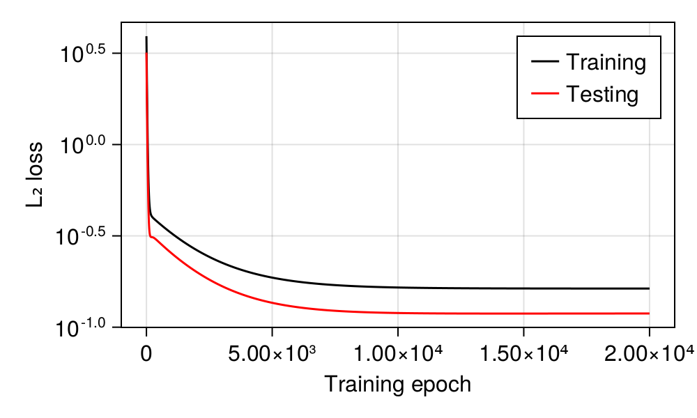
We are producing the loss over time figure after the training, as it is good practice – but as we mentioned in the previous section, it is very common to have the training code look at the dynamics of these two values in order to decide whether to stop the training early.
Before moving forward, let’s look at Figure 3.2 a little more closely. In the first steps, the loss decreases very rapidly – this is because we started from a value of \(\mathbf{\beta}\) that is, presumably, far away from the optimum, and therefore the gradient is really strong. Despite the low learning rate, we are making long steps in the space of parameters. After this initial rapid increase, the loss decreases much more slowly. This, counter-intuitively, indicates that we are getting closer to the optimum! At the exact point where \(\beta_0\) and \(\beta_1\) optimally describe our dataset, the gradient vanishes, and our system would stop moving. And as we get closer and closer to this point, we are slowing down. In the next section, we will see how the change in loss over times ties into the changes with the optimal parameter values.
3.4.5 Visualizing the learning process
From Figure 3.3, we can see the change in \(\beta_0\) and \(\beta_1\), as well as the movement of the current best estimate of the parameters (right panel). The sharp decrease in loss early in the training is specifically associated to a rapid change in the value of \(\beta_0\). Further note that the change in parameters values is not monotonous! The value of \(\beta_1\) initially increases, but when \(\beta_0\) gets closer to the optimum, the gradient indicates that we have been moving \(\beta_1\) in the “wrong” direction.
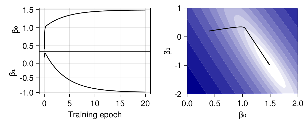
This is what gives rise to the “elbow” shape in the right panel of Figure 3.3. Remember that the gradient descent algorithm, in its simple formulation, assumes that we can never climb back up, i.e. we never accept a costly move. The trajectory of the parameters therefore represents the path that brings them to the lowest point they can reach without having to temporarily recommend a worse solution.
But how good is the solution we have reached?
3.4.6 Outcome of the model
We could read the performance of the model using the data in Figure 3.2, but what we really care about is the model’s ability to tell us something about the data we initially gave it. This is presented in Figure 3.4. As we can see, the model is doing a rather good job at capturing the relationship between the number of species and the number of interactions.
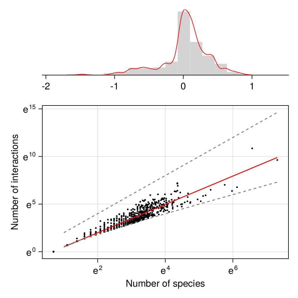
We will have a far more nuanced discussion of “what is this model good for?” in Chapter 4, but for now, we can make a decision about this model: it provides a good approximation of the relationship between the species richness, and the number of interactions, in a food web.
3.5 A note on regularization
One delicate issue that we have avoided in this chapter is the absolute value of the parameters. In other words, we didn’t really care about how large the model parameters would be, only the quality of the fit. This is (generally) safe to do in a model with a single parameter. But what if we had many different terms? What if, for example, we had a linear model of the form \(\hat y \approx \beta_0 + \beta_1 x + \beta_2 x^2\)? What if our model was of the form \(\hat y \approx \beta_0 + \beta_1 x + \dots + \beta_n x^n\)? What if \(n\) started to get very large compared to the number of data points?
In this situation, we would very likely see overfitting, wherein the model would use the polynomial terms we provided to capture more and more noise in the data. This would be a dangerous situation, as the model will lose its ability to work on unknown data!
To prevent this situation, we may need to use regularization. Thanfkully, regularization is a relatively simple process. In Equation 3.4, the function \(f(p)\) we used to measure the gradient was the loss function directly. In regularization, we use a slight variation on this, where
\[ f(p) = \text{loss} + \lambda \times g(\beta) \,, \]
where \(\lambda\) is an hyper-parameter giving the strength of the regularization, and \(g(\beta)\) is a function to calculate the total penalty of a set of parameters.
When using \(L1\) regularization (LASSO regression), \(g(\beta) = \sum |\beta|\), and when using \(L2\) regularization (ridge regression), \(g(\beta) = \sum \beta^2\). When this gets larger, which happens when the absolute value of the parameters increases, the model is penalized. Note that if \(\lambda = 0\), we are back to the initial formulation of the gradient, where the parameters have no direct effect on the cost.
3.6 Conclusion
In this chapter, we have used a dataset of species richness and number of interactions to start exploring the practice of machine learning. We defined a model (a linear regression), and based about assumptions about how to get closer to ideal parameters, we used the technique of gradient descent to estimate the best possible relationship between \(S\) and \(L\). In order to provide a fair evaluation of the performance of this model, we kept a part of the dataset hidden from it while training. In Chapter 4, we will explore this last point in great depth, by introducing the concept of cross-validation, testing set, and performance evaluation.
References
Brose, Ulrich, Annette Ostling, Kateri Harrison, and Neo D. Martinez. 2004. “Unified Spatial Scaling of Species and Their Trophic Interactions.” Nature 428 (6979): 167–71. https://doi.org/10.1038/nature02297.
Cohen, J. E., and F. Briand. 1984. “Trophic Links of Community Food Webs.” Proc Natl Acad Sci U S A 81 (13): 4105–9.
Innes, Michael. 2018. “Don’t Unroll Adjoint: Differentiating SSA-Form Programs.” https://doi.org/10.48550/ARXIV.1810.07951.
MacDonald, Arthur Andrew Meahan, Francis Banville, and Timothée Poisot. 2020. “Revisiting the Links-Species Scaling Relationship in Food Webs.” Patterns 1 (0). https://doi.org/10.1016/j.patter.2020.100079.
Martinez, Néo D. 1992. “Constant Connectance in Community Food Webs.” The American Naturalist 139 (6): 1208–18. http://www.jstor.org/stable/2462337.
Morrison, Margaret, and Mary S. Morgan. 1999. “Models as Mediating Instruments.” In, 10–37. Cambridge University Press. https://doi.org/10.1017/cbo9780511660108.003.