7 Hyper-parameters tuning
In Chapter 3, we represented the testing and training loss of a model as a function of the number of gradient descent steps we had made. This sort of representation is very useful to figure out how well our model is learning, and is called, appropriately enough, a learning curve. We further discussed that the learning rate (and possibly the regularization rate), and the number of epochs, where hyper-parameters of the model. An hyper-parameter is usually defined as a parameter of the model that is controlling the learning process, but is not itself modified through learning (Yang and Shami 2020). Hyper-parameters usually need to be determined before the training starts (Claesen and De Moor 2015), but there are various strategies to optimize them. In this chapter, we will produce learning curves to find the optimal values of hyper-parameters of the model we developed in Chapter 5 and Chapter 6.
We will illustrate this using an approach called moving-threshold classification, and additionally explore how we can conduct searches to tune several hyper-parameters at once. There are many techniques to sample multiple parameters at the same time, including Latin hypercube sampling (Huntington and Lyrintzis 1998), orthogonal sampling (McKay, Beckman, and Conover 1979), and grid searches. The common point to all of these approaches are that they generate a combination of hyper-parameters, which are used to train the model, and measures of performance are then used to pick the best possible combination of hyper-parameters. In the process of doing this, we will also revisit the question of why the MCC is a good measure of the classification performance, as well as examine tools to investigate the “right” balance between false/true positive rates. At the end of this chapter, we will have produced a very good model for the distribution of the Corsican nuthatch, which we will then explain in Chapter 8.
7.1 Classification based on probabilities
When first introducing classification in Chapter 5 and Chapter 6, we used a model that returned a deterministic answer, which is to say, the name of a class (in our case, this class was either “present” or “absent”). But a lot of classifiers return quantitative values, that correspond to (proxies for) the probability of the different classes. Nevertheless, because we are interested in solving a classification problem, we need to end up with a confusion table, and so we need to turn a number into a class. In the context of binary classification (we model a yes/no variable), this can be done using a threshold for the probability.
Note that the quantitative value returned by the classifier does not need to be a probability; it simply needs to be on an interval or ratio scale.
The idea behind the use of thresholds is simple: if the classifier output \(\hat y\) is larger than (or equal to) the threshold value \(\tau\), we consider that this prediction corresponds to the positive class (the event we want to detect, for example the presence of a species). In the other case, this prediction corresponds to the negative class. Note that we do not, strictly, speaking, require that the value \(\hat y\) returned by the classifier be a probability. We can simply decide to pick \(\tau\) somewhere in the support of the distribution of \(\hat y\).
The threshold to decide on a positive event is an hyper-parameter of the model. In the NBC we built in Chapter 5, our decision rule was that \(p(+) > p(-)\), which when all is said and done (but we will convince ourselves of this in Section 7.3.1), means that we used \(\tau = 0.5\). But there is no reason to assume that the threshold needs to be one half. Maybe the model is overly sensitive to negatives. Maybe there is a slight issue with our training data that bias the model predictions. And for this reason, we have to look for the optimal value of \(\tau\).
There are two important values for the threshold, at which we know the behavior of our model. The first is \(\tau = \text{min}(\hat y)\), for which the model always returns a negative answer; the second is, unsurprisingly, \(\tau = \text{max}(\hat y)\), where the model always returns a positive answer. Thinking of this behavior in terms of the measures on the confusion matrix, as we have introduced them in Chapter 5, the smallest possible threshold gives only negatives, and the largest possible one gives only positives: they respectively maximize the false negatives and false positives rates.
7.1.1 The ROC curve
This is a behavior we can exploit, as increasing the threshold away from the minimum will lower the false negatives rate and increase the true positive rate, while decreasing the threshold away from the maximum will lower the false positives rate and increase the true negative rate. If we cross our fingers and knock on wood, there will be a point where the false events rates have decreased as much as possible, and the true events rates have increased as much as possible, and this corresponds to the optimal value of \(\tau\) for our problem.
We have just described the Receiver Operating Characteristic (ROC; Fawcett (2006)) curve! The ROC curve visualizes the false positive rate on the \(x\) axis, and the true positive rate on the \(y\) axis. The area under the curve (the ROC-AUC) is a measure of the overall performance of the classifier (Hanley and McNeil 1982); a model with ROC-AUC of 0.5 performs at random, and values moving away from 0.5 indicate better (close to 1) or worse (close to 0) performance.The ROC curve is a description of the model performance across all of the possible threshold values we investigated!
7.1.2 The PR curve
One very common issue with ROC curves, is that they are overly optimistic about the performance of the model, especially when the problem we work on suffers from class imbalance, which happens when observations of the positive class are much rarer than observations of the negative class. In ecology, this is a common feature of data on species interactions (Poisot et al. 2023). In addition, although a good model will have a high ROC-AUC, a bad model can get a high ROC-AUC too (Halligan, Altman, and Mallett 2015); this means that ROC-AUC alone is not enough to select a model.
An alternative to ROC is the PR (for precision-recall) curve, in which the positive predictive value is plotted against the true-positive rate; in other words, the PR curve (and therefore the PR-AUC) quantify whether a classifier makes reliable positive predictions, both in terms of these predictions being associated to actual positive outcomes (true-positive rate) and not associated to actual negative outcomes (positive predictive value). Because the PR curve uses the positive predictive values, it captures information that is similar to the ROC curve, but is in general more informative (Saito and Rehmsmeier 2015).
7.1.3 A note on cross-entropy loss
In Chapter 3, we used loss functions to measure the progress of our learning algorithm. Unsurprisingly, loss functions exist for classification tasks too. One of the most common is the cross-entropy (or log-loss), which is defined as
\[ −\left[y \times \text{log}\ p+(1−y)\times \text{log}\ (1−p)\right] \,, \]
where \(y\) is the actual class, and \(p\) is the probability associated to the positive class. Note that the log-loss is very similar to Shannon’s measure of entropy, and in fact can be expressed based on the Kullback-Leibler divergence of the distributions of \(y\) and \(p\). Which is to say that log-loss measures how much information about \(y\) is conveyed by \(p\). In this chapter, we use measures like the MCC that describe the performance of a classifier when the predictions are done, but log-loss is useful when there are multiple epochs of training. Neural networks used for classification commonly use log-loss as a loss function; note that the gradient of the log-loss function is very easy to calculate, and that gives it its usefulness as a measure of learning.
7.2 How to optimize the threshold?
In order to understand the optimization of the threshold, we first need to understand how a model with thresholding works. When we run such a model on multiple input features, it will return a list of probabilities, for example \([0.2, 0.8, 0.1, 0.5, 1.0]\). We then compare all of these values to an initial threshold, for example \(\tau = 0.05\), giving us a vector of Boolean values, in this case \([+, +, +, +, +]\). We can then compare this classified output to a series of validation labels, e.g. \([-, +, -, -, +]\), and report the performance of our model. In this case, the very low thresholds means that we accept any probability as a positive case, and so our model is very strongly biased. We then increase the threshold, and start again.
As we have discussed in Section 7.1, moving the threshold is essentially a way to move in the space of true/false rates. As the measures of classification performance capture information that is relevant in this space, there should be a value of the threshold that maximizes one of these measures. Alas, no one agrees on which measure this should be (Perkins and Schisterman 2006; Unal 2017). The usual recommendation is to use the True Skill Statistic, also known as Youden’s \(J\) (Youden 1950). The biomedical literature, which is quite naturally interested in getting the interpretation of tests right, has established that maximizing this value brings us very close to the optimal threshold for a binary classifier (Perkins and Schisterman 2005). In a simulation study, using the True Skill Statistic gave good predictive performance for models of species interactions (Poisot 2023).
Some authors have used the MCC as a measure of optimality (Zhou and Jakobsson 2013), as it is maximized only when a classifier gets a good score for the basic rates of the confusion matrix. Based on this information, Chicco and Jurman (2023) recommend that MCC should be used to pick the optimal threshold regardless of the question, and I agree with their assessment. A high MCC is always associated to a high ROC-AUC, TSS, etc., but the opposite is not necessarily true. This is because the MCC can only reach high values when the model is good at everything, and therefore it is not possible to trick it. In fact, previous comparisons show that MCC even outperform measures of classification loss (Jurman, Riccadonna, and Furlanello 2012).
For once, and after over 15 years of methodological discussion, it appears that we have a conclusive answer! In order to pick the optimal threshold, we find the value that maximizes the MCC. Note that in previous chapters, we already used the MCC as a our criteria for the best model, and now you know why.
7.3 Application: improved Corsican nuthatch model
In this section, we will finish the training of the model for the distribution of Sitta whiteheadi, by picking optimal hyper-parameters, and finally reporting its performance on the testing dataset. At the end of this chapter, we will therefore have established a trained model, that we will use in Chapter 8 to see how each prediction emerges.
7.3.1 Making the NBC explicitly probabilistic
In Chapter 5, we have expressed the probability that the NBC recommends a positive outcome as
\[ P(+|x) = \frac{P(+)}{P(x)}P(x|+)\,, \]
and noted that because \(P(x)\) is constant across all classes, we could simplify this model as \(P(+|x) \propto P(+)P(x|+)\). But because we know the only two possible classes are \(+\) and \(-\), we can figure out the expression for \(P(x)\). Because we are dealing with probabilities, we know that \(P(+|x)+P(-|x) = 1\). We can therefore re-write this as
\[ \frac{P(+)}{P(x)}P(x|+)+\frac{P(-)}{P(x)}P(x|-) = 1\, \]
which after some reorganization (and note that \(P(-) = 1-P(+)\)), results in
\[ P(x) = P(+) P(x|+)+P(-) P(x|-) \,. \]
This value \(P(x)\) is the “evidence” in Bayesian parlance, and we can use this value explicitly to get the prediction for the probability associated to the class \(+\) using the NBC.
Note that we can see that using the approximate version we used so far (the prediction is positive if \(P(+) P(x|+) > P(-) P(x|-)\)) is equivalent to saying that the prediction is positive whenever \(P(+|x) > \tau\) with \(\tau = 0.5\). In the next sections, we will challenge the assumption that \(0.5\) is the optimal value of \(\tau\).
In Figure 7.1, we show the effect of moving the threshold from 0 to 1 on the value of the MCC. This figure reveals that the value of the threshold that maximizes the average MCC across folds is \(\tau \approx 0.43\). But more importantly, it seems that the “landscape” of the MCC around this value is relatively flat – in other words, as long as we do not pick a threshold that is too outlandishly low (or high!), the model would have a good performance. It is worth pausing for a minute and questioning why that is.
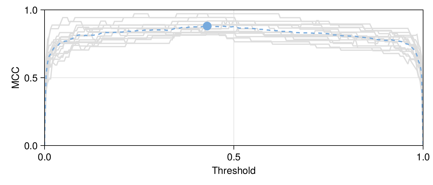
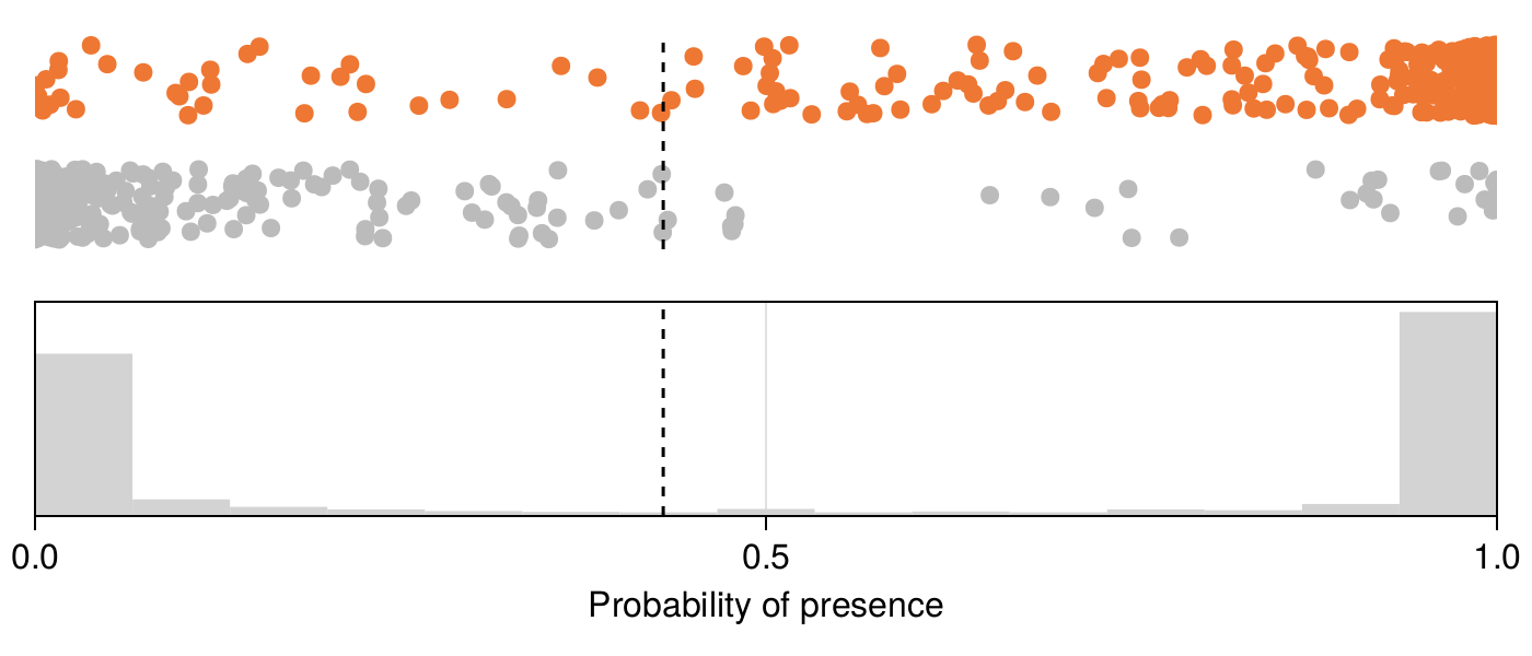
To do so, we can look at the distribution of probabilities returned by the NBC, which are presented in Figure 7.2. It appears that the NBC is often confident in its recommendations, with a bimodal distribution of probabilities. For this reason, small changes in the position of the threshold would only affect a very small number of instances, and consequently only have a small effect on the MCC and other statistics. If the distribution of probabilities returned by the NBC had been different, the shape of the learning curve may have been a lot more skewed.
7.3.2 How good is the model?
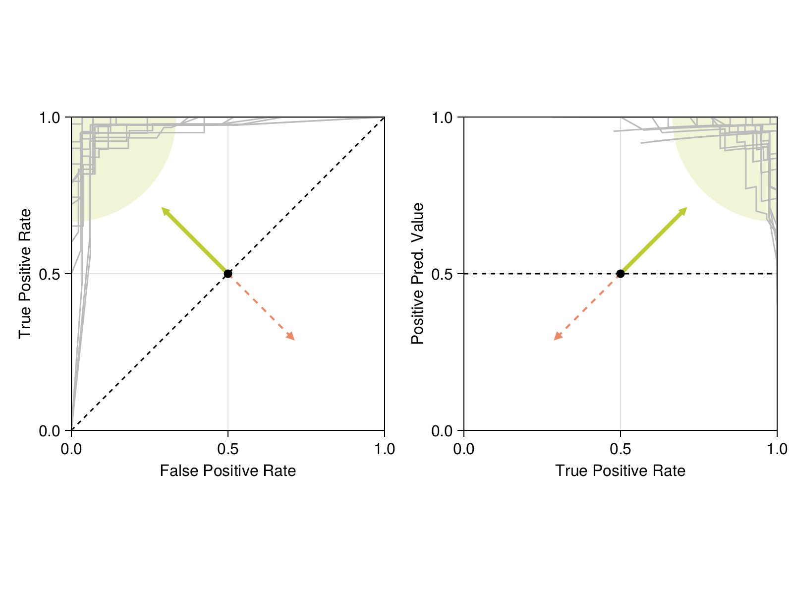
After picking a threshold and seeing how it relates to the distribution of probabilities in the model output, we can have a look at the ROC and PR curves. They are presented in Figure 7.3. In both cases, we see that the model is behaving correctly (it is nearing the point in the graph corresponding to perfect classifications), and importantly, we can check that the variability between the different folds is low. The model also outperforms the no-skill classifier. Taken together, these results give us a strong confidence in the fact that our model with the threshold applied represents an improvement over the version without the threshold.
7.3.3 Fine-tuning the NBC prior
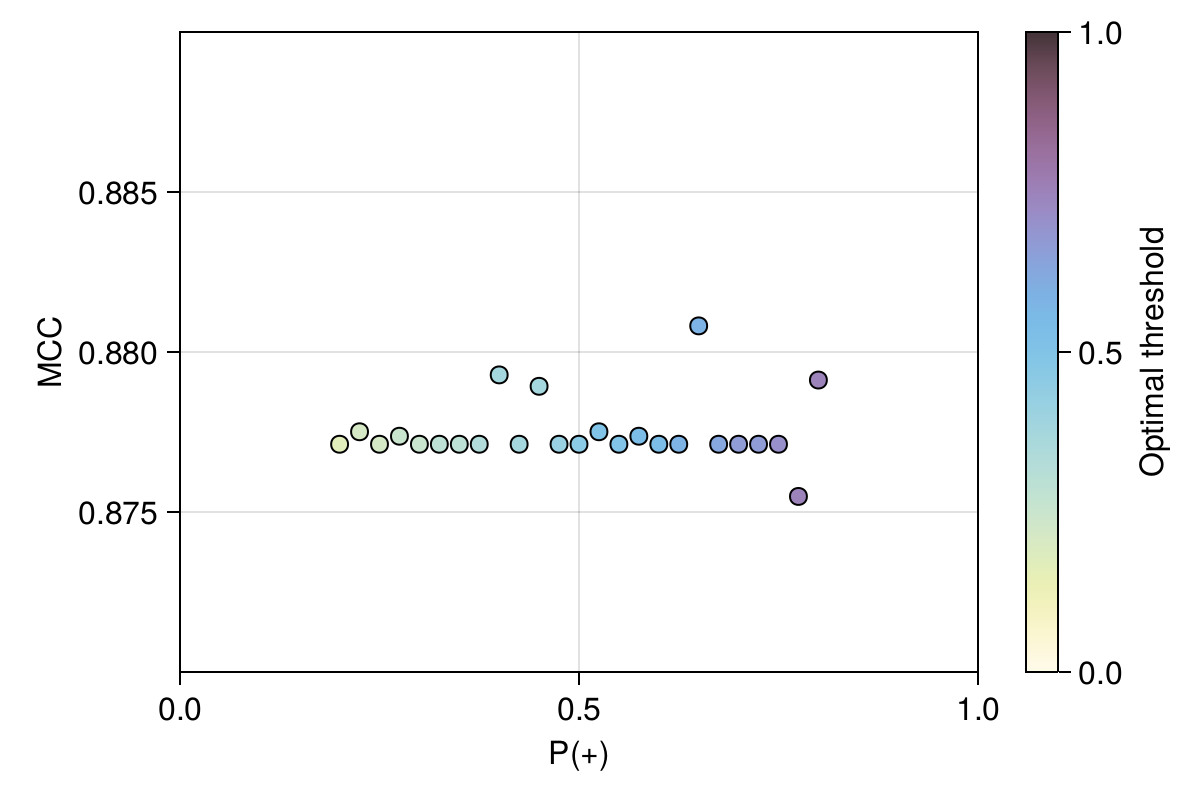
In the previous section, we have assumed that the prior on occurrences \(P(+)\) was one half, which is a decision we can revisit. But changing this value would probably require that we also change the threshold, and for this reason we need to optimize both hyperparameters at the same time. We present the results of a simple grid search in Figure 7.4.
Based on these results, it appears that changing the value of the prior has very little impact on the best MCC we can achieve: the threshold is simply adjusted to reflect the fact that we assume occurrences to be increasingly likely. In this example, there is very little incentive for us to change the value of the prior, as it would have a very small effect on the overall performance of the model. For this reason, we will keep the previous model (\(P(+) = 0.5\) and \(\tau \approx 0.43\)) as the best one.
A grid search in an exhaustive sweep of all possible combinations of parameter values. In order to make the process more efficient, refined approaches like successive halvings (Jamieson and Talwalkar 2016) can be used.
Just because we decided to use a learning curve does not mean we have to change the hyper-parameters. Sometimes, this approach reveals that the value of an hyper-parameter is not really important to model performance, and we need to make a decision on what to do next. Here, although there are marginal changes in the value of the MCC, they do not feel significant enough to change the value of the prior.
7.3.4 Testing and visualizing the final model
As we are now considering that our model is adequately trained, we can apply it to the testing data we had set aside early in Chapter 5. Applying the trained model to this data provides a fair estimate of the expected model performance, and relaying this information to people who are going to use the model is important.
We are not applying the older versions of the model to the testing data, as we had decided against this. We had established the rule of “we pick the best model as the one with the highest validation MCC”, and this is what we will stick to. To do otherwise would be the applied machine learning equivalent of \(p\)-hacking, as the question of “what to do in case a model with lower validation MCC had a better performance on the testing data?” would arise, and we do not want to start questioning our central decision this late in the process.
We can start by taking a look at the confusion matrix on the testing data:
\[ \begin{pmatrix} 153 & 12 \\ 4 & 105 \end{pmatrix} \]
This is very promising! There are far more predictions on the diagonal (258) than outside of it (16), which suggests an accurate classifier. The MCC of this model is 0.881, its true-skill statistic is 0.872, and its positive and negative predictive values are respectively 0.927 and 0.963. In other words: this model is extremely good. The values of PPV and NPV in particular are important to report: they tell us that when the model predicts a positive or negative outcome, it is expected to be correct more than 9 out of 10 times.
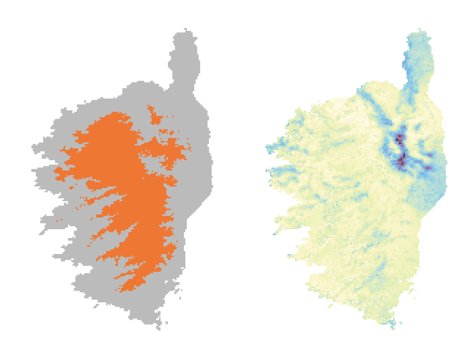
The final predictions are shown in Figure 7.5. Although the range map is very similar to the one we produced by the end of Chapter 6, the small addition of an optimized threshold leads to a model that is overall a little more accurate. Note that the uncertainty has a much nicer spatial structure when compared to our initial attempt (in Figure 5.4): there are combinations of environmental variables that make prediction more difficult, but they tend to be very spatially clustered.
7.4 Conclusion
In this chapter, we have refined a model by adopting a principled approach to establishing hyper-parameters. This resulted in a final trained model, which we applied to produce the final prediction of the distribution of Sitta whiteheadi. In Chapter 8, we will start asking “why”? Specifically, we will see a series of tools to evaluate why the model was making a specific prediction at a specific place, and look at the relationship between the importance of variables for model performance and for actual predictions.